Stock Market Predictions
Ray has been working on a number of predictive algorithms that take past data and try to extrapolate into the future. Ray has applied some of these algorithms to the stock market. With the background and publication provided here, everyone can go back and check and see how well the algorithms performed.
Methodology
The response of a specific stock index can be thought of as the response of a classical second order system. But you wouldn't want the system that you are modeling to be represented by a single second order system because then the response would be a simple, damped sine wave. And we know the stock market does not behave like this. So we compose the model of the stock market as the sum of 10 (for example) second order systems with different natural frequencies of oscillation and damping ratios.
The response of these systems would be known except that you don't know the input forcing function. Thus the matching/predictive algorithm has to determine the best estimate of the forcing function so that each second order system response can be determined. Thus another variable at each "time slice" can be thrown into the mix along with the natural frequency of each second order system and the damping ratio of each second order system.
Data
The last ten years of monthly closing data for the Dow Jones Industrial Average (DJIA), the NASDAQ (IXIC), and the Standard and Poors 500 (SPX) indices were grabbed from Yahoo financial historical data. This data has all of the appropirate "adjustments" in the monthly closing prices.
The data, 120 monthly closing prices for each index, were presented to the matching alogrithm in order to determine the best natural frequency and damping ratio of each second order system, as well as a forcing function "input" value for each of the 120 monthly periods.
The matching alogirhtm goes off to crunch numbers to find the best fit parameters for a summed second order system to match the actual stock index monthly closing price. The "best fit" fitness function was a root-sum-squared (RSS) difference between the actual index closing price and the predictive algorithm closing price. The iterative optimization process takes a while to perform, but in the end a set of parameters is derived that "matches" the historical data in an RSS manner.
DJIA Matching Results
The matching results of the algorithm are shown below in Figure 1 for the DJIA. In this case, the actual closing average is shown in blue compared with the matching algorithm results in red. The matching algorithm misses some of the higher frequency content of the DJIA closing response but captures the essence of its movement. Recall that the matching algorithm has derived natural frequencies and damping ratios for each second order system as well as the required "external" inputs needed to produce the DJIA response.
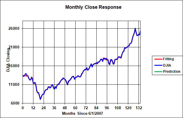
Figure 1. DJIA Closing Actual Against Matched
Figure 1 probably looks a lot like a 30 day moving average of the DJIA but without the time lag. This would not be correct. The red "predictive" line is not a moving average but rather a matching of the 10 or so second order systems to past DJIA monthly close data. There is no averaging taking place except for the fact that none of the data is daily data. It is all monthly close data.
Figure 2 shows the resulting the "external" inputs to the system. These "external" inputs represent the forcing function for each of 120 months as a result of global events, events within the United States, reporting of corporate earnings, and other inputs that could effect the movement of the DJIA. It is not intended to break down where these inputs came from or what they are attributed to. It is only needed to derive what these values are to match the DJIA monthly closing price.
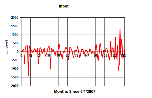
Figure 2. External Forcing Function
DJIA Predictive Results
The prediction (or extrapolation) of the stock market response cannot be performed without an input forcing function that goes along with each month that is going to predicted. But we don't know what the future forcing functions are. In the absence of better knowledge, a Monte Carlo analysis is performed where the natural frequencies and damping ratios of each oscillator is fixed (at the previosuly-determined optimum) and the prior forcing function values are also fixed. The Monte Carlo analysis is performed for future month forcing functions using the average and standard deviation of the previously-derived forcing functions that were used to match past data.
This methodology allows us to determine an average response for future months as well as an expected range (provided future month forcing function values are not radically different than the past).
Figure 3 shows a typical set of predictions for the month closing prices beyond the original DJIA time history. It can be seen that the predicted closing price can vary a moderate amount depending upon the alignment of future month forcing functions as derived in the Monte Carlo analysis. Nonetheless, as of 24 June 2017 using data up to 1 June 2017, 6 and 12 month average DJIA closing values would be 21687 (1 December 2017) and 20861 (1 June 2018). Figure 4 shows the histogram of closing prices for the DJIA for 500 Monte Carlo runs. Again the 12 month ahead closing price clusters near 20861.
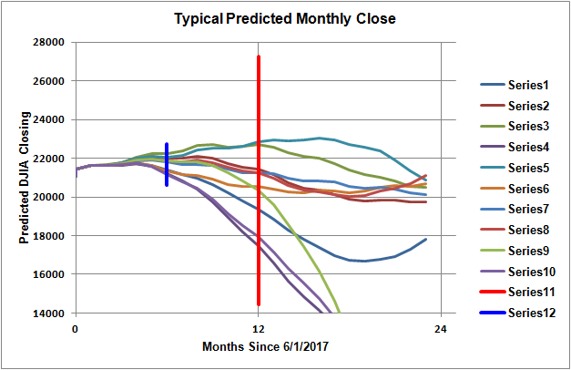
Figure 3. Typical 24 Month Ahead DJIA Closing Prices
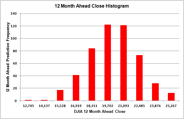
Figure 4. Twelve Month Ahead DJIA Close Price Histogram, 500 Runs
The same process as described above for the DJIA was applied to the NASDAQ index. It should be boted that the natural frequencies and damping ratios of each second order system are different between the DJIA and NASDAQ results (since the historical curves to be matched are different). Furthermore the optimized forcing function values for the 120 month historical period are different between the two indices. One way to look at this is that the indices are made up of different component stocks and would be affected by global or national or emergency events in different ways.
NASDAQ Matching Results
The matching results of the algorithm are shown below in Figure 5 for the NASDAQ index. In this case, the actual closing average is shown in blue compared with the matching algorithm results in red. The matching algorithm misses some of the higher frequency content of the NASDAQ closing response but captures the essence of its movement. Recall that the matching algorithm has derived natural frequencies and damping ratios for each second order system as well as the required "external" inputs needed to produce the NASDAQ response.
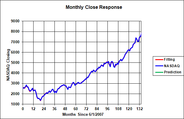
Figure 5. NASDAQ Closing Actual Against Matched
NASDAQ Predictive Results
The prediction (or extrapolation) of the NASDAQ followed the same procedure described above for the DJIA. Namely, a Monte Carlo analysis was performed where random forcing functions for the future 24 months were applied and the responses computed. Five hundred Monte Carlo runs were made.
Figure 6 shows a typical set of predictions for the month closing prices beyond the original NASDAQ time history. It can be seen that the predicted closing price can vary a moderate amount depending upon the alignment of future month forcing functions as derived in the Monte Carlo analysis. Nonetheless, as of 24 June 2017 using data up to 1 June 2017, 6 and 12 month average NASDAQ closing values would be 6228 (1 December 2017) and 5869 (1 June 2018).
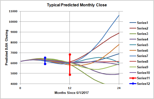
Figure 6. Typical 24 Month Ahead NASDAQ closing Prices
Prediction Summary
| Closing Date | ||||||
| 12/1/2017 | Prediction Actual | 21687 24232 |
Prediction Actual | 6228 6848 |
Prediction Actual | 2388 2642 |
| 6/1/2018 | Prediction Actual | 20861 24271 |
Prediction Actual | 5869 7510 |
Prediction Actual | 2143 2718 |
| 12/1/2018 | Prediction Actual | 41813 |
Prediction Actual | 6599 |
Prediction Actual | 3854 |